Chimera: An Open Source RNA Pipeline for Long Covid Research
Back in October, I found out about a new initiative in Europe called Amatica Health. Instead of regular blood tests for long covid, which I have tons and tons of, they were offering a RNA sequencing covering over 20,000 genes that was hopefully going to shed some light on the entire disease and maybe lead to a cure.
I paid the $1000 (or whatever it was at the time), and submitted my sample. In the time between then and when I received my results, I shared a few emails and X messages with some of the founders. Some of the things I was curious about was just how much juice we can squeeze from the RNA data set. After some back and forth with one of the founders, I decided to try and write a 'simple' RNA pipeline I could run on a dedicated server I have at home that was meant for doing AI experiments.
I was given my raw FASTQ file from my initial run, which I used to validate this. Since that time, Amatica has spoken to their GDPR and legal reps etc and decided that releasing their full CSV of raw data, calibrated to their controls, was equivalent/better than releasing the FASTQs - as such, they are no longer able to release patient FASTQ files. I won't comment on that except to say that it's their internal decision, and I'm at least fortunate that I had my n=1 data file to experiment with. In truth, processing a RNA sample is no small feat, and there is nothing really plug and play about it. Having a raw data dump of 30,000 GENEs in a CSV file calibrated against a control cohort (which Amatica provides) is also valuable and informative for most people.
Since I spent about 200 hours putting this pipeline together, I do want to at least talk about my efforts as I'm convinced tools like this can help the research community. As such, this post will highlight some of the challenges I faced with running my own sample, and where I see this project going next (since I can't finish it with just one sample).
This project is called Chimera, and it's an open-source (eventually) RNA pipeline for long covid + me/cfs research.
Controls
When you process an RNA file in a bioinformatics pipeline, you generally end up with a pile of subdirectories full of data. All of this is hard to interpret and on its own and is sort of meaningless in isolation. What you really need to do is say, "how does this data compare to a group that is healthy?"
Amatica is solving this problem internally by running their own controls (healthy people) through their exact same pipeline. That's the ideal setup, as there aren't really any batch effects (things you have to account for if the two groups were processed differently).
Since I don't have access to their controls (for obvious reasons), what I needed was a series of FASTQ files from healthy people I could process on my own. And it turns out there are lots of great data sets for this purpose available publicly.
I did some research and found a few public groups that match these, one of which was GSE217948, an Australian pandemic control set with 70 healthy volunteers. These were all ribo depleted (as opposed to polya) with approximately 100M paired reads. Perfect.
Calibration
The problem with calibrating against a control set run via a different process is due to batch effects. You usually account for these by comparing a batch of unhealthy people against a batch of controls. You can then do some mathematical voodoo to try and match the distributions better and remove these batch effects to better compare.
The problem was I didn't have a batch of unhealthy people, I just had me. So how do you calibrate one person's RNA sample against and entire cohort of healthy people run on a different sequencer and likely with different prep methods?
My solution to this was two fold:
- Separate the problem into protein encoding genes vs non protein encoding genes. Then recalibrate the counts per million (TPM) based on this data. In effect it's a normalization step to make TPM comparable for the coding genes. This method seemed to bring the means and the variance more inline with each other, which is what I was hoping.
- Find a set of 100 - 200 housekeeping genes - genes that don't really move all that much between healthy people and unhealthy people. Use these to calibrate between the two data sets. This was the second process I did.
Once I had my actual Amatica data, I planned to see if my TPM/z-scoring matched theirs - it mostly did: 92% matched in terms of general direction, the ones that didn't were mostly genes close to 0 with a lot of noise. So I was and am confident that the protein encoding GENE parts of the pipeline mostly match and are trustworthy.
What To Test
I used AI to help me assemble the entire pipeline, mostly like a kid assembling tinker toy. I wanted the pipeline to be able to process both RNA sequencing data and Whole Genome Sequencing (WGS) data. To do that on a local machine requires about 300GB of reference data to be downloaded, including alignment info for the entire human genome. That was the first step, mostly assembling the various reference files.
The second was doing a big exploration about what was possible, relying heavily on AI to help fill in the gaps. I'm an engineer, not a bioinformatics person, so I had to do a lot of research about what was possible. Every time I read a paper over the last few weeks that related to long covid, I modified my pipeline to be able to look for it. Paper after paper, new code after new code, the whole pipeline eventually came together.
Internally I have something called a signature, which is a fingerprint based on GENES, directions, pathology, sub-scoring etc, that can be configured with a basic yaml file. So for every hypothesis, I can basically bake it into a signature yaml, and simple run that one stage again. That meant I could iterate quickly whenever I wanted to test something different For example, here is a signature configuration file for inflammatory cytokines:
# Cytokine & chemokine signature panel definitions — 10 panels.
# Sub-panels grouped by functional role, independently scored and z-scored.
# Gene overlap across panels is intentional (e.g., IL1B in proinflammatory + inflammasome).
# Pure data: gene lists, ratios, categories. No display strings.
# Display text lives in run/layers/config/annotations.yaml.

  # ---------------------------------------------------------------------------
  # Core cytokine axis panels (10)
  # ---------------------------------------------------------------------------

  cyto_proinflammatory:
    category: cytokine
    display_name: "Pro-Inflammatory Cytokines"
    pathological_direction: up
    genes:
      - IL1B
      - IL6
      - TNF
      - IL12A
      - IL12B
      - IL18
      - IL23A
      - OSM
      - LIF
      - HMGB1
    references:
      - pmid: "32546811"
        citation: "Del Valle et al. 2020, Nat Med 26(10):1636-1643"
        title: "An inflammatory cytokine signature predicts COVID-19 severity and survival"
        contribution: "IL-6, TNF, IL-1beta as predictors of COVID-19 severity and mortality"
This is no regular machine - it has 64GB of DDR5 memory, and the pipeline with controls is maxed out at 2TB of data. It has 28 cores, and even with that it takes between 60 and 90 minutes to run a single sample. Running the entire control cohort from scratch is days, not hours. So this isn't something that can be run easily on a regular laptop or desktop machine - it needs some heavy resources or a cloud based processing pipeline.
LOO Control References
Everything that a patient goes through in terms of the pipeline, the controls go through as well. During the final stage of the control part though, when I'm building my master data file representing the contol cohort, I also add a second stage where I score each control against the entire control cohort as well, minus themselves. This is called leave-one-out scoring, and it's meant to see how controls score against each other. This allows me to come up with a scoring mechanism for all my signatures - not only are the gene directions pathological according to my signature yaml definition, but how serious is the deviation compared to controls who were scored the same way. So basically everything in the pipeline can be z-scored using this method, not just individual genes, but every composite score as well.
Usability
I got tired pretty quick of manually running CLI commands every time I wanted to run or ru-run a patient or control, so I added a web based admin panel to Chimera.
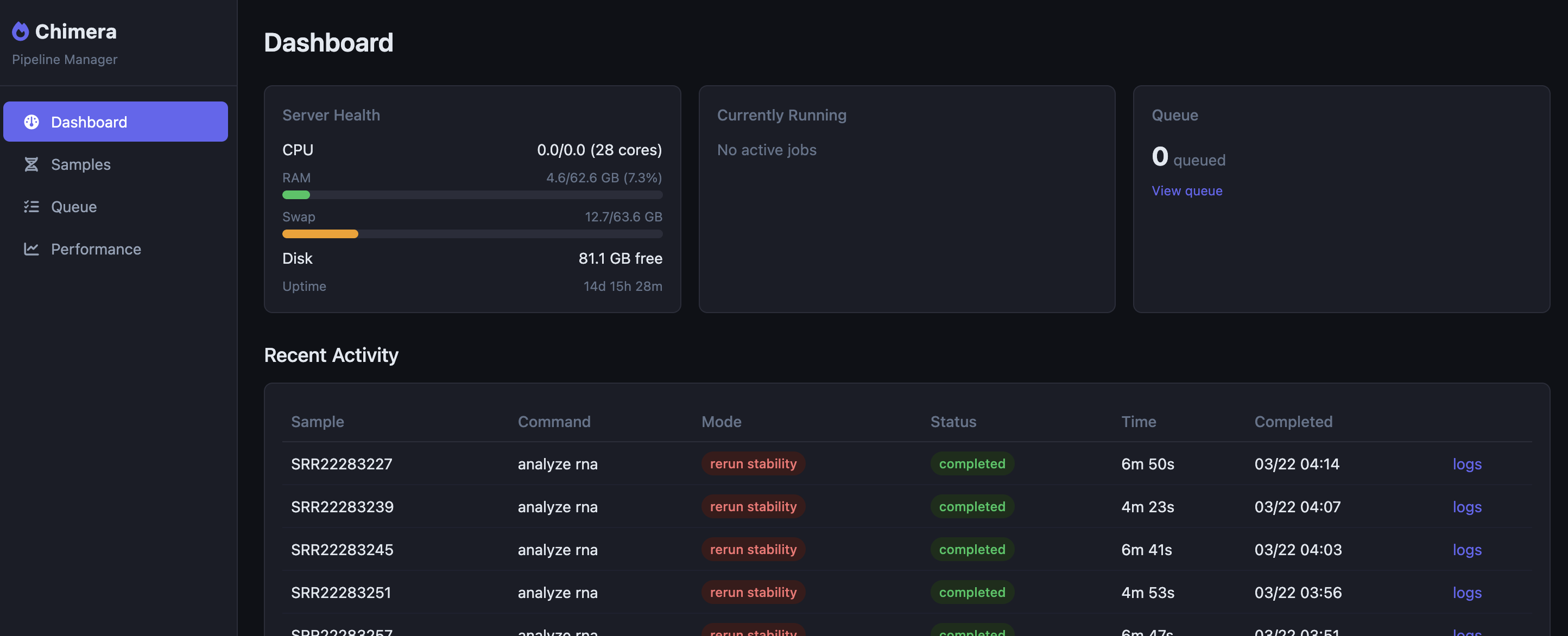
This dashboard has a queue system which lets me queue individual stages or even entire runs, all with a few clicks. Updating my signature files, for example, requires that I run the entire signature pipeline for each person again. This takes about 10 seconds per sample, so for 70 controls and one patient it's a quickish 710 seconcds.
Results
Ok, now for the fun stuff. I'm going to take you through all the things that I baked into the pipeline. This is all n=1, so nothing here should be taken as anything other than demonstrating the viability of having a private RNA pipeline you can control yourself.
Flow Cytometry
One of the first interesting tools I hooked up was immune cell deconvolution. It's basically like a poor person's flow cytometry test. There are various algorithms that can be used to estimate the amount of immune cells in a sample. Since each algorithm on its own was noisy, I added four different algorithms to the pipeline and they also output how well they agree. The goal was to show which results you can likely trust and which ones were likely less trustworthy.
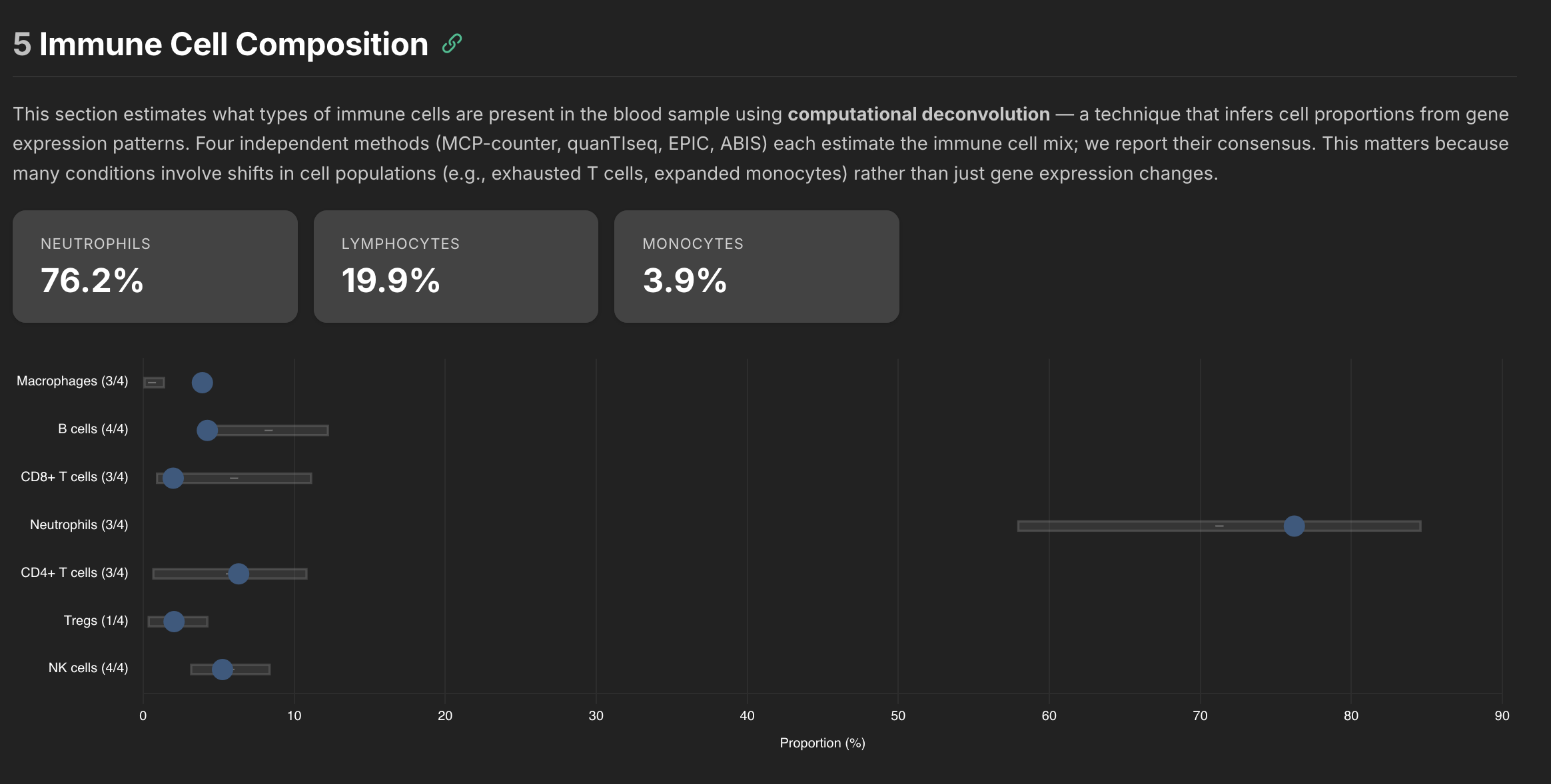
Here was the raw data from the pipeline along with how each compared to the control cohort.
| Category | Sub-type | Cell Type | Proportion (%) | Methods | Z-Score | Status |
|---|---|---|---|---|---|---|
| Neutrophils | 76.2 | 3/3 | ▲ +0.44 (ref: 71.3 ± 13.4) | Normal range | ||
| Lymphocytes | 19.9 | |||||
| CD4+ T cells | 6.3 | 3/3 | ▲ +0.33 (ref: 5.7 ± 5.1) | Normal range | ||
| naive | 9.92 | 1/1 | ▼ -0.95 | Normal range | ||
| MAIT cells | 9.92 | 1/1 | ▼ -0.61 | Normal range | ||
| memory | 8.29 | 1/1 | ▼ -0.11 | Normal range | ||
| Gamma-delta T cells | 2.86 | 1/1 | +0.00 | Normal range | ||
| CD8+ T cells | 2.0 | 3/4 | ▼ -0.84 (ref: 6.0 ± 5.1) | Normal range | ||
| naive | 3.43 | 1/1 | ▲ +1.72 | Mildly elevated | ||
| memory | 0.00 | 1/1 | ▼ -1.58 | Mildly suppressed | ||
| B cells | 4.3 | 4/4 | ▼ -1.37 (ref: 8.3 ± 4.0) | Normal range | ||
| memory | 2.89 | 1/1 | ▼ -0.40 | Normal range | ||
| naive | 1.37 | 1/1 | ▼ -1.47 | Normal range | ||
| Plasma cells | 0.08 | 1/1 | ▲ +1.07 | Normal range | ||
| NK cells | 5.3 | 4/4 | ▲ +0.04 (ref: 5.8 ± 2.6) | Normal range | ||
| Monocytes | Monocytes | 0.0 | 1/3 ⚠ | ▲ +3.09 (ref: 0.0 ± 0.0) | Markedly elevated vs. reference | |
| classical | 8.06 | 1/1 | ▼ -1.28 | Normal range | ||
| non-classical | 2.19 | 1/1 | ▼ -0.07 | Normal range | ||
| Macrophages | 3.9 | 3/3 | ▲ +3.09 (ref: 0.6 ± 0.8) | Markedly elevated vs. reference | ||
| M2 | 3.91 | 1/1 | ▲ +3.09 | Markedly elevated vs. reference | ||
| M1 | 0.00 | 1/1 | ▲ +3.09 | Markedly elevated vs. reference | ||
| Basophils | 32.3 | 1/1 | ▲ +2.19 | Notably elevated | ||
| Dendritic Cells | Dendritic cells | 0.00 | 2/3 | ▲ +2.19 (ref: 0.0 ± 0.0) | Notably elevated | |
| Non-Hematologic (deconvolution artifacts) | Uncharacterized | 0.0 | 1/2 ⚠ | ▲ +3.09 (ref: 0.0 ± 0.0) | Markedly elevated vs. reference |
Some of the cells like naive B cells only are estimated using 1 of the 4 algorithms, so those are flagged as less reliable. But as you can see there is a lot of data there. One of the defining characteristics about what is going on in my body is a high neutrophil to lymphocyte ratio (NLR). When I was very symptomatic it was around 10, and it typically hovers around 4-5 these days. That matches what came out of this pipeline, so it seems reasonable at least to my known blood tests.
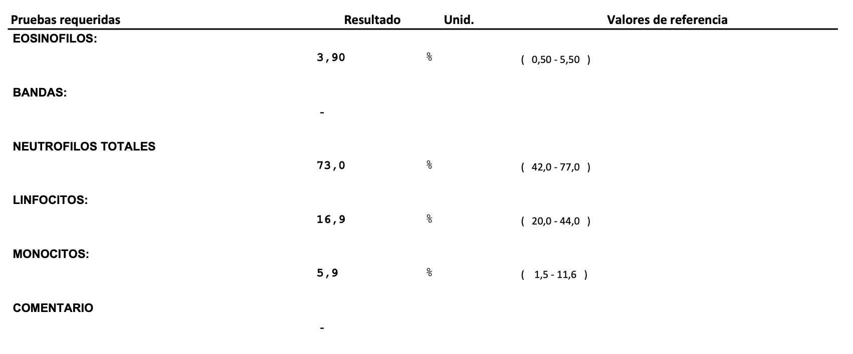
If you compare against an actual CBC I had done around the same time as this draw, they are in pretty close agreement. The difference is the cell deconvolution gives you much more information about the cell subsets.
Signatures
Every signature's internal metrics (GENES etc) gets scored against the control cohort, as well as the entire signature panel itself. In my reporting system, this is how it looks.
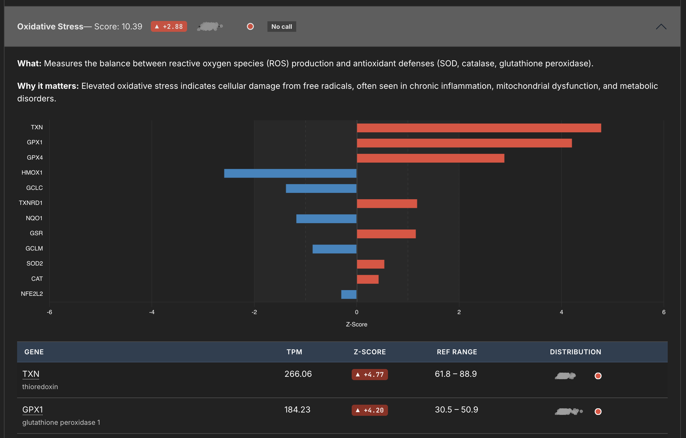
This panel measures Oxidative Stress, and you can see from the little sparkline (I thought being able to visually see the distribution would be cool) where this signature matches against the whole. You can also see the breakdown of the individual genes below.
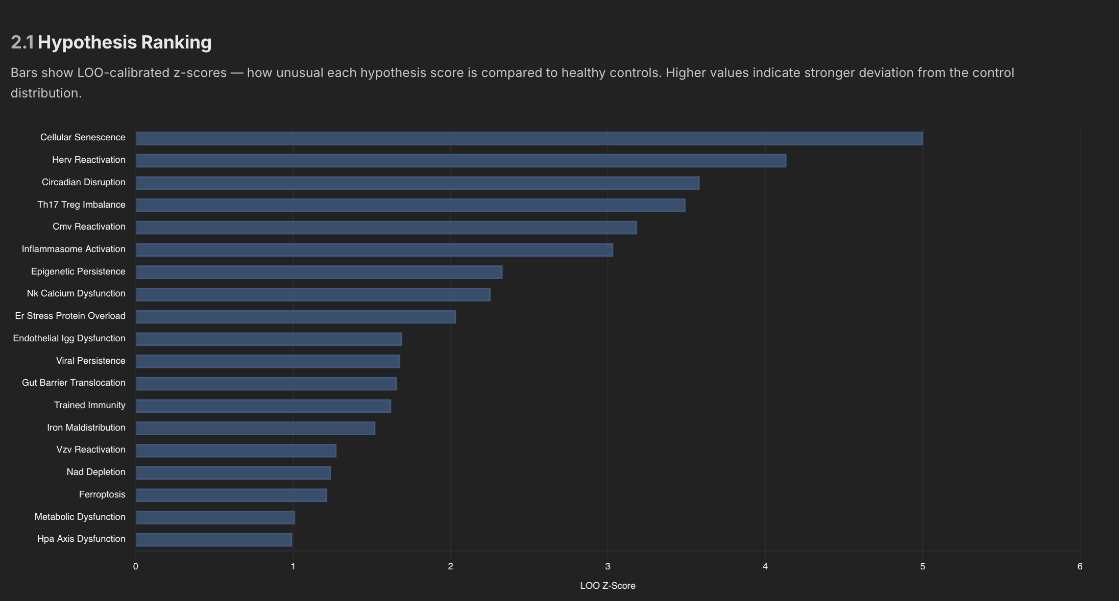
Internally I have about 100 signatures or more I think, and many of those signatures are then aggregated into overarching hypothesis, which also get ranked against controls as well.
Pathogen Detection
I have an entire pipeline section detected to pathogen detection - it can detected both viruses and bacteria (depending on the sample). I wasn't sure what useful data this might produce, so this was an experiment.
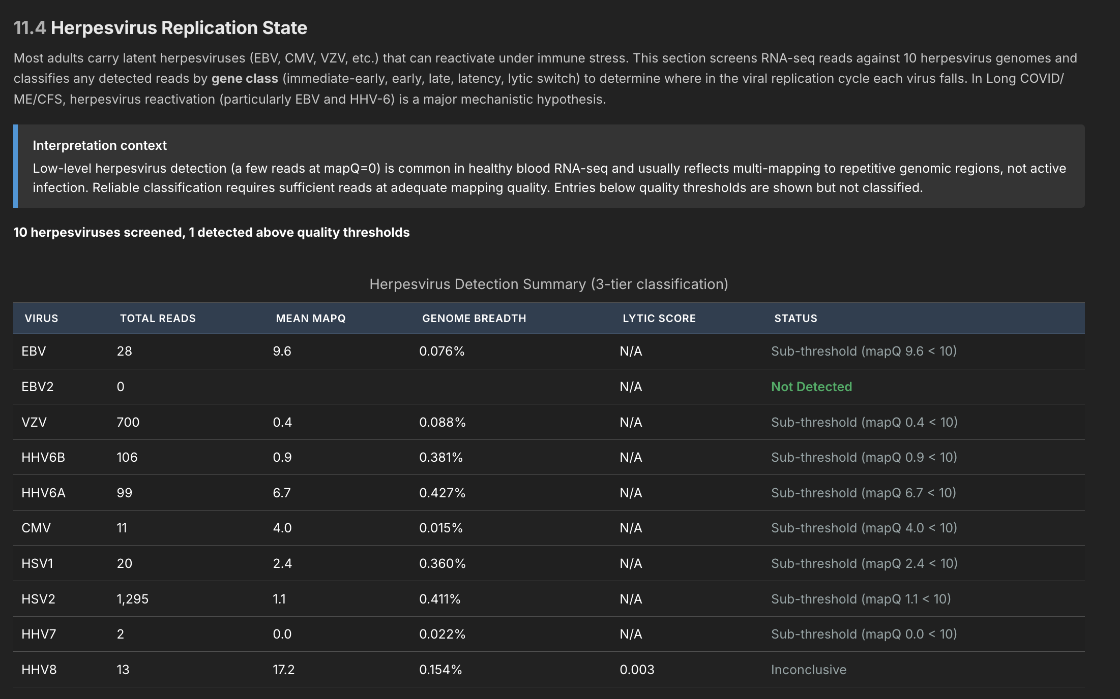
The pathogen detection pipeline has three independent stages, meant to filter out noise at each stage. Since I only tested myself and healthy controls, I haven't really been able to verify it's working (although I did get a pretty conclusive multi-level match that one of the controls had hepatitis C). In general this was a good exercise, but until I test more data I can't be confident it can find anything in blood (expressions might be too small). But the machinery is all hooked up to detect about 180 different viruses known to be associated with ME/CFS, as well as all herpesviruses.
RNA Editing
There are probably 20 or more stages to the pipeline, each outputting interesting data on its own. Here's one that might be relevant in terms of Long Covid - the RNA editing rate.
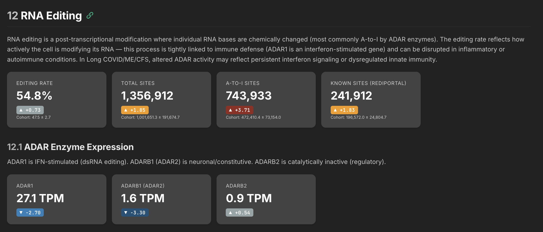
The RNA editing rate tells you whether your cells are keeping up with the job of defusing self-generated false alarms. ADAR enzymes edit double-stranded RNA that the cell produces naturally — without this editing, the immune system mistakes its own RNA for a viral infection and triggers inflammation. The problem can go two ways: either the editing enzymes are too low and can't keep up, or the volume of RNA needing editing is so high that even normal enzyme levels would fall behind.
My interpretation of my own data is this: my ADAR enzymes are suppressed but my actual editing rate is elevated — which sounds contradictory until you realize it means there's so much more substrate being produced that even depleted enzymes are generating above-normal editing activity. The enzyme is losing a race against an overwhelming volume of self-derived dsRNA. The editing system is working harder than normal and still falling behind.
Exonic Ratios
This was a stage I added just as a proof of concept, but I quickly came to realize its importance. RNA is mostly a photograph of what is going on at a particular point in time in a person's body. You can see what genes are expressed, but you don't typically know what they're doing. The intronic/exonic ratio tells you more though.
If a gene's expression level is its position — a snapshot of where it is right now — the intronic ratio is its velocity, telling you which direction it's heading. Is the gene ramping up, coasting on old transcript, or being actively held back? A gene can look normal in a snapshot but be heading off a cliff, or look suppressed but actually be fighting hard to recover. Without the velocity information, you'd never know.
Asking AI to review this one dataset, it says the following:
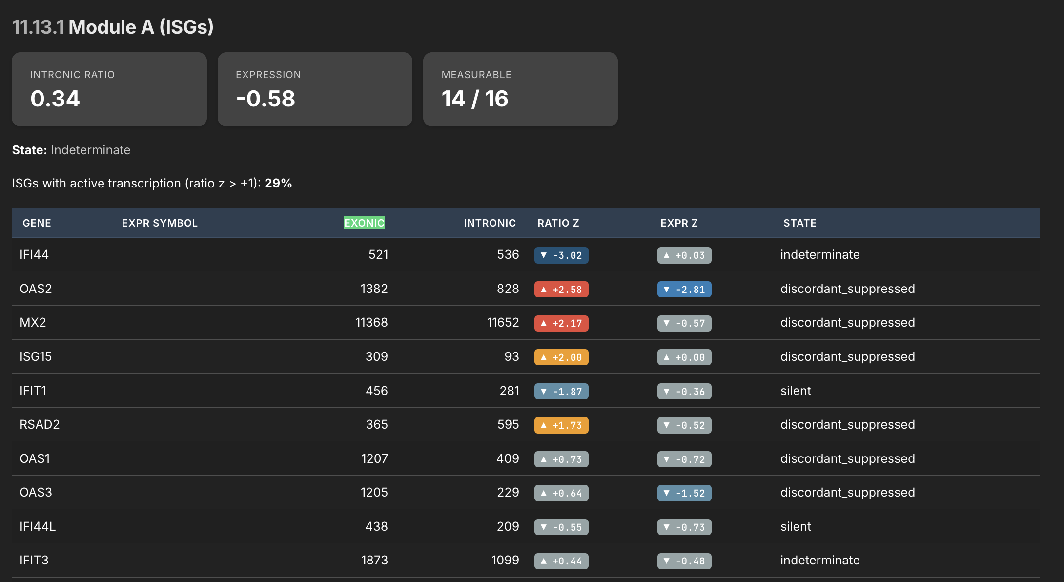
This is the intronic/exonic ratio analysis — the viral persistence plausibility module. The logic: intronic reads indicate active transcription right now (unspliced pre-mRNA), while exonic reads capture both new and old stable mRNA. The ratio between them tells you whether a gene is being actively driven or just coasting on accumulated transcript. The pattern here is stark and specific. Look at the "discordant_suppressed" genes:
- OAS2 — ratio z=+2.58, expression z=-2.81. This is the most alarming single line in the table. The cell is actively transcribing OAS2 at a rate 2.58 standard deviations above normal. But the mature mRNA level is 2.81 standard deviations below normal. The cell is making OAS2 pre-mRNA aggressively, but the finished product isn't accumulating. That transcript is being destroyed after it's made, or blocked before it matures. OAS2 is an interferon-stimulated RNase that degrades viral RNA — it's one of the key effectors of the antiviral response.
- MX2 — ratio z=+2.17, expression z=-0.57. Same pattern, slightly milder. Active transcription of this GTPase that blocks viral nuclear import. The cell is trying. The output is suppressed.
- ISG15 — ratio z=+2.00, expression z=+0.00. The cell is driving ISG15 transcription at double the normal rate, and all that effort produces... exactly normal expression. Whatever is destroying or blocking the mRNA is absorbing all of the extra transcriptional output. ISG15 conjugates to viral proteins to restrict their function — it's a direct antiviral effector.
- RSAD2/viperin — ratio z=+1.73, expression z=-0.52. Another actively transcribed antiviral effector that isn't accumulating. Viperin disrupts viral replication by producing ddhCTP, a chain terminator for viral RNA-dependent RNA polymerase.
- OAS1 and OAS3 — both showing positive ratio z scores (+0.73, +0.64) with suppressed expression (-0.72, -1.52). The entire OAS family is being driven but not producing output. OAS3 is particularly notable — expression z=-1.52 is a meaningful deficit.
This data is useful if you're trying to develop a hypothesis about whether something is actively blocking the immune response in real time — not just that the immune system is weak, but that it's actively trying and being intercepted. The cell is sending the signal, the genes are responding, the transcription machinery is working — but the finished product never arrives. That's a very different picture from simple immune suppression, and it's exactly what I was trying to use this module to detect.
HERV Expression
One thing I learned during this exercise is that our DNA is very old. It's like a record of our entire evolutionary history, and even contains some very old machinery long since rendered inactive by natural selection. So basically our own DNA encodes many super ancient viruses (specifically retroviruses and retrotransposons).
Normally our body silences all of these genes such that they can't cause us harm. But some of the working theories in MS and ME/CFS revolve around these elements. In theory, if the specific molecular machinery that keeps these elements silenced gets disrupted enough, these ancient retro elements could re-express themselves and you would have your own body essentially producing foreign material.
These elements are called Human Endogenous Retroviruses, and my pipeline was set up to try and quantify them.
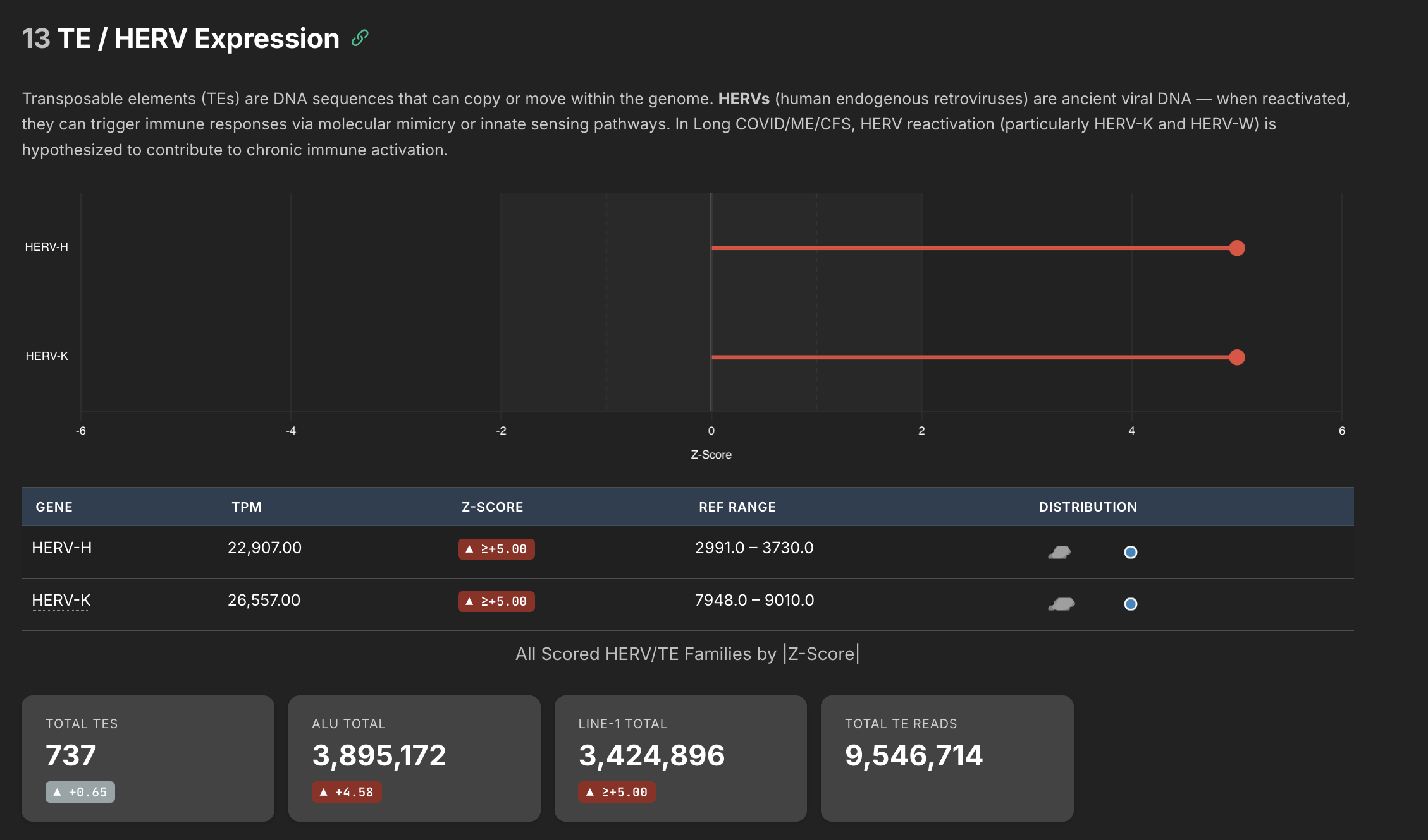
This is the data I'm the least confident about in my pipeline, so I wouldn't place too much weight on what we are seeing here. I detected a staggeringly high amount of HERVs in my own sample, but there are clearly batch effects going on that I can't account for yet. The key insight is that HERVs and HERV based effects can be quantified using this pipeline, and might be able to provide insight into whether HERVs are actually expressing themselves meaningfully in long covid and ME/CFS patients.
The cascade would mostly be:
- initial virus disrupts the HERV silencing machinery
- the suppression damages the mechanism that holds HERVs at bay
- HERVs begin re-expressing themselves - your body is literally making foreign material at this stage
- Foreign HERVs basically get treated like foreign viruses, and your body reacts the same way - fighting against a pathogen
- If this mechanism goes on too long, the machinery that silences these things may shut off for good - it becomes self sustaining.
- When this cascade starts, the clock starts ticking in terms of the body's ability to reverse it
Note: If you were looking for a hypothesis for Long COVID, this is a compelling one — is viral persistence actually SARS-CoV-2 still in the body, or is the persistence more about ancient retroelements that are no longer being silenced? It could be either, or both, and the ratio might differ between patients. If HERV derepression is a significant contributor, it would explain why antivirals directed at the virus itself show inconsistent results — you're treating the trigger but not the self-sustaining mechanism it left behind. I've seen some evidence so far that it may involve the latter. But that's an open hypothesis I think worth exploring.
BCR/TCR Repertoire
This is actually the section that surprised me the most. I was a little disappointed when the pathogen detection pipeline didn't produce much, but there turned out to be a lot of signal hiding in the BCR/TCR data. BCR and TCR are the receptors on B cells and T cells — they're the molecular fingerprints that tell you which specific immune clones are present and what they might be targeting.
The sequencer captures fragments of these receptors, and using various pipeline tools you can reconstruct a list of all the heavy chains and light chains that were picked up during the run. When the body makes an antibody against a pathogen, it combines a heavy chain and a light chain together — the pair forms the specific shape that locks onto the target. The limitation with this approach is that while the pipeline can detect heavy chains and light chains independently, there's no way to determine the exact pairing from short-read RNA-seq data.
This matters because the same heavy chain paired with different light chains can target completely different things. Without that pairing information, a lot of what you're seeing is still noise. But it's hypothesis-generating noise — you can identify which immune gene families are expanded, spot oligoclonal patterns that suggest the immune system is reacting to something specific, and flag candidate clones worth investigating further with more targeted methods.
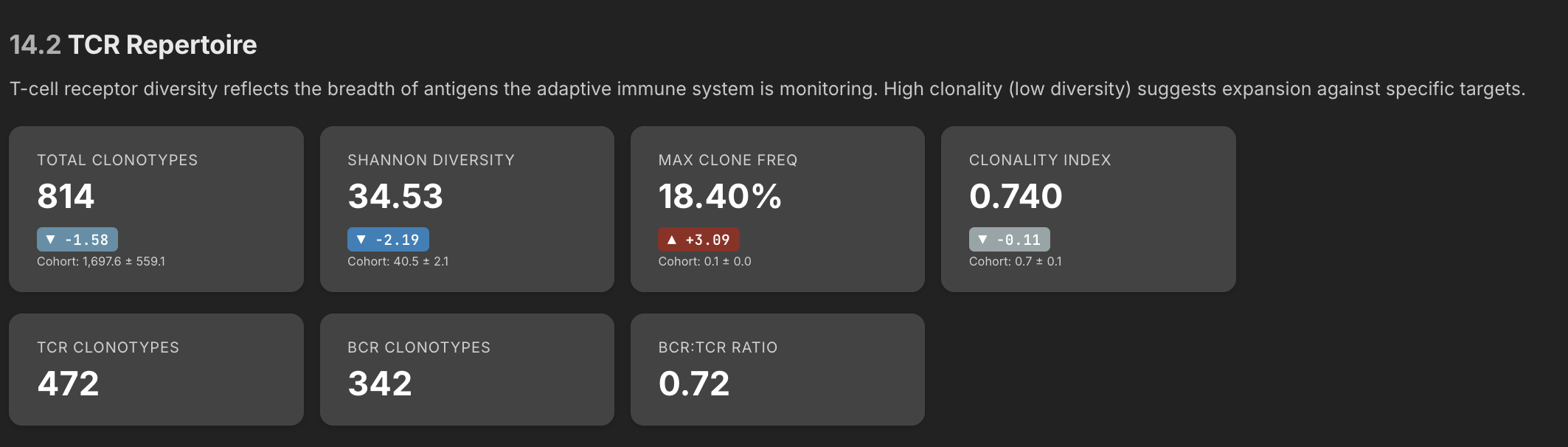
One thing that immediately jumped out in the data is I have a one clone that represents 18.4% of all my clones - that's exceptionally high. In most people clonal frequencies are more like 1-3%. The fact that one clone is pegged this high shows that my overall repertoire has contracted, and one particular clone has expanded. A single clone at 18.4% means my immune system has devoted nearly one in five of its B cell resources to fighting one thing. This might be a sign of active antibody engagement against one particular target.
Here is the raw data, showing the expanded clone at the top:
| Chain | CDR3 AA | V Gene | J Gene | SHM | Count | Frequency |
|---|---|---|---|---|---|---|
| IGH | CDYYYYYGMDVW | IGHV3-15*03 | IGHJ6*02 | 40 | 18.40% | of all IGH |
| IGK | CQQYYSTPPWTF | IGKV4-1*01 | IGKJ1*01 | 11 | 3.78% | of all IGK |
| IGL | CAAWDDSLSGWVF | IGLV1-47*01 | IGLJ3*02 | 7 | 2.41% | of all IGL |
| IGK | CMQALQTPRF | IGKV2-28*01 | IGKJ3*01 | 7 | 2.41% | of all IGK |
| IGL | CQAWDSSTSVVF | IGLV3-1*01 | IGLJ2*01 | 6 | 2.06% | of all IGL |
| IGH | CARDSHHYDILTGSAGDFDYW | IGHV1-3*01 | IGHJ4*02 | 6 | 2.70% | of all IGH |
| IGK | CMQATHWRMF | IGKV2-30*02 | IGKJ1*01 | 6 | 2.06% | of all IGK |
| IGH | CAKVPITMIVVGTRKRNNWFDPW | IGHV3-23*01 | IGHJ5*02 | 5 | 2.25% | of all IGH |
| IGK | CQQYNNWPQYTF | IGKV3-15*01 | IGKJ2*01 | 5 | 1.72% | of all IGK |
| IGH | CARGPKITMVRGVIVDYW | IGHV1-8*01 | IGHJ4*02 | 5 | 2.25% | of all IGH |
| IGK | CQQSYSTPHTF | IGKV1-39*01 | IGKJ1*01 | 4 | 1.68% | of all IGK |
| IGH | CARESTNIVVVVAATRGDYFDYW | IGHV3-30*03 | IGHJ4*02 | 4 | 1.80% | of all IGH |
| IGK | CQQADSFPITF | IGKV1D-12*01 | IGKJ5*01 | 4 | 1.37% | of all IGK |
The SHM (somatic hypermutation) count tells you something important about how mature a clone is. When a B cell encounters a target, it enters structures in the lymph nodes called germinal centers, where it undergoes rounds of mutation and selection — each round slightly refines the antibody's fit against the target, like iteratively sharpening a key to better fit a lock. Each round leaves mutations behind in the DNA. An SHM count of 40 on my dominant clone means it has been through extensive refinement — this isn't a B cell that just woke up last week. It's been actively engaging a target for a long time, getting better and better at binding it. For comparison, the other heavy chain clones in my data have SHM counts of 4-6, which is much more typical.
Reading this data as objectively as I can, three things stand out:
-
There is a persistent antigen. Something has been present in the body long enough for a B cell to go through dozens of rounds of affinity maturation against it. An SHM of 40 isn't consistent with something that came and went — it's consistent with something that's been there for months or longer, continuously stimulating the immune system.
-
The immune system considers it a priority. At 18.4% of all heavy chain clones, the body has devoted a disproportionate share of its B cell resources to this one target. That level of commitment means whatever this clone is targeting, the immune system has decided it matters more than maintaining a diverse repertoire against other potential threats.
-
The response is mature but hasn't resolved. In a normal immune response, you encounter a pathogen, expand clones against it, clear the pathogen, and the expanded clones contract back to a small memory population. A clone still dominating at 18.4% with 40 SHMs means the target hasn't been cleared — either it's still there, or the immune system thinks it's still there. A resolved response shouldn't look like this.
A dominant clone like this has a short differential — it could indicate a persistent antigen driving an immune response, an autoimmune expansion, or in the worst case, a lymphoproliferative process like lymphoma. The high somatic hypermutation count and the presence of other diverse clones make the last option unlikely — malignant clones tend to expand because they've lost growth control, not because they're chasing an antigen, so they typically show lower SHM.
So my best guess is this indicates an ongoing immune response against something that has been there long enough for the B cells to go through 40 rounds of maturation — and whatever it is, it hasn't been cleared yet.
Closing Thoughts
As you can see, there is a ton of data you can get out of an RNA sample. There are probably 10 pipeline stages I haven't talked about here, but they all produce different viewpoints of the same data, which together can be used to generate hypotheses.
Unfortunately for me, I've only tested one sample, so it's hard to further refine the pipeline. My goal was to release this to the public so that research institutions could use it for some of their own analysis, but with n=1 I don't have enough data to refine it and fix bugs. So for now I'm mostly in a holding pattern.
That said, I have contacted several RNA labs, one of which has agreed to help support this effort - I'll be sending them some more of my blood soon which they've agreed to run for me at a super high resolution, about 2x the amount of data I've so far had for my own blood, so I can further refine this.
I also have the entire unhealthy controls from that long covid control cohort as well. That dataset is really interesting because each patient has multiple FASTQ files representing their journey through the hospital during their acute phase. Some of them, sadly, even died. Using some of my pipeline tools I should be able to see each of their journeys at a RNA level from acute to resolved or acute to deceased, That might shed some light on why some people recover and why some don't. I have enough signals in my own RNA to have formed four of five hypotheses in my own head about what might be going on, some of which I haven't seen discussed in the research literature yet. So I'll be able to explore those ideas soon.
The goal for me is to eventually open this on GitHub for researchers to use. But at this point I'm several months off, and need more data. But thanks to my new relationship with an actual RNA lab, one of which is enthusiastic about what I've shown them, I should hopefully have some more data to work with soon.